How is Energy Storage Capacity Calculated?

Getting energy storage capacity right is one of the most consequential decisions in any BESS project. Undersize it, and you leave critical use cases unserved. Oversize it, and you lock capital into stranded assets. Yet capacity calculation is frequently reduced to a rough rule of thumb — “we need X hours of backup, so install Y kWh” — that ignores the real interaction between power demand peaks, energy throughput requirements, degradation trajectories, and cycle economics.

This guide provides a rigorous, application-tested framework. It begins with the fundamental three-step calculation method, then applies it to specific deployment scenarios, and finally covers the advanced planning levers that separate bankable, long-lived systems from underperforming ones.

I. Prerequisite for capacity calculation: Accurately defining electricity demand.

Daily average electricity consumption can be calculated as follows: Residential users can calculate their consumption through electricity bills or smart meters, typically ranging from 5-20 kWh per day; industrial and commercial users need to record electricity consumption data for each production period, and their daily average consumption can reach hundreds or even thousands of kWh depending on their scale.

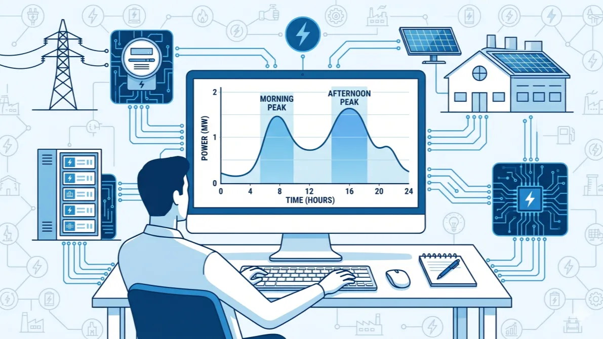
Analyzing peak and valley electricity consumption characteristics reveals that electricity demand is not uniformly distributed. Residential electricity consumption typically peaks in the morning and evening, while industrial and commercial electricity consumption exhibits a unique curve following production rhythms (e.g., peak daytime production electricity consumption in factories and low nighttime equipment maintenance electricity consumption). Understanding these peak and valley patterns is crucial for determining the discharge power requirements of energy storage systems and the optimal timing for intervention.

Assess backup power requirements: In areas with unstable power supply (such as remote areas) or scenarios with high requirements for power continuity (such as medical equipment, production lines, and data centers), additional backup capacity is needed. This is typically designed to be 50%-100% of the average daily power consumption, with the specific percentage depending on the user’s tolerance for power outages (e.g., in medical settings where power outage tolerance is extremely low, the backup ratio needs to be close to 100%).

II. Core Method: Three-Step Calculation Method for Energy Storage Capacity

Step 1: Calculate the basic capacity

The basic capacity needs to be determined by considering average daily electricity consumption, reserve requirements, and peak-valley differences, as shown in the following formula:

Basic capacity = Average daily electricity consumption × Reserve factor (1.5-2.0, corresponding to 50%-100% reserve demand) × Peak correction factor (1.0-1.1 for residential users, 1.1-1.3 for industrial and commercial users, due to greater peak-valley differences in industrial and commercial users).

Example: A household consumes an average of 10 kWh of electricity per day and requires 50% as reserve. Using a peak power correction factor of 1.1, the base capacity is 10 × 1.5 × 1.1 = 16.5 kWh.

Step 2: Adjust the actual capacity

Batteries exhibit “incomplete discharge” characteristics, and energy loss occurs during system operation, necessitating adjustments to the base capacity.

Actual capacity = Base capacity ÷ (Depth of discharge × System efficiency) Depth of discharge (DOD): Lithium iron phosphate batteries typically use 80%-90% (shallow charging and discharging can extend battery life);

System efficiency: Includes charging and discharging losses, inverter conversion efficiency, line losses, etc., typically 85%-95% (high-quality systems can achieve efficiencies of over 90%).

Example: With a base capacity of 16.5 kWh, a depth of discharge of 85%, and a system efficiency of 92%, the actual capacity = 16.5 ÷ (0.85 × 0.92) ≈ 21.1 kWh

Step 3: Design the final capacity (including safety margin)

To address battery degradation (capacity decreases with long-term use), extreme weather (such as insufficient photovoltaic power generation due to continuous rain), and unexpected load increases (such as the addition of temporary equipment), a safety margin needs to be increased.

Final capacity = Actual capacity × (1 + safety margin)

A safety margin is typically 10%-20%, but the specific margin should be determined based on the usage environment (e.g., batteries degrade faster in high/low temperature regions, so the margin can be increased appropriately) and the expected lifespan (e.g., if planned for 10 years, a 20% margin is recommended).

Example: With an actual capacity of 21.1 kWh, adding a 15% safety margin, the final capacity = 21.1 × 1.15 ≈ 24.3 kWh (the actual configuration can be taken as 24 kWh).

III. Capacity Planning Strategies for Different Scenarios

The formula provides the mathematical answer. But the inputs — and the critical checks — differ substantially by use case and scale. Below are planning strategies for the four most common BESS scenarios.

Scenario 1 — Residential Backup Power

Planning approach: The goal is to power essential loads through an outage, not the entire house.

1. Audit critical loads only: Identify refrigerators, medical devices, lighting, routers, and HVAC as essential. Exclude entertainment systems, ovens, and workshop equipment.
2. Sum critical load wattage and multiply by desired backup hours to get Erequired.
3. Apply the Step 2–3 formula. Residential LFP systems (e.g., 48V architecture) typically operate at 80–90% DoD with 85–90% RTE.
4. Size for peak simultaneous startup loads, not average wattage. Motor-driven loads (pumps, compressors) draw 3–6× rated wattage at startup, which determines the required power rating (kW), not the energy (kWh).

Typical scale: 5–30 kWh, paired with a 3–15 kW inverter.

Common pitfall: Sizing for average consumption rather than critical loads leads to oversizing that never pays back. Conversely, failing to identify a powered subpanel with non-essential circuits can unexpectedly drain a correctly sized battery.

Scenario 2 — Commercial & Industrial (C&I) Peak Shaving

Planning approach: Peak shaving is fundamentally a power-led (kW) sizing problem, not an energy problem. The objective is to cap the highest 15-minute demand interval on the utility bill.

1. Obtain 12 months of 15-minute interval meter data. Identify the highest power demand spike and the typical duration of the peak window.
2. Define the shaving target — the power threshold below which all billing demand should fall (e.g., cut all spikes above 500 kW).
3. Calculate required power (kW): PBESS=Ppeak−Pthreshold
4. Calculate required energy (kWh): Multiply the power delta by the typical peak duration. Example: 200 kW reduction for 1.5 hours = 300 kWh.
5. Apply the DoD/RTE/margin correction from Steps 2–3 of the core formula.
6. Verify C-rate compatibility: Peak shaving often demands 1C or higher discharge rates. Confirm the selected cells and PCS support this rate at the required duration.

Typical scale: 100 kWh to 10 MWh with 50–500 kW PCS.

Key metric: C&I systems typically achieve 20–50% peak load reduction, translating directly into lower grid fees.

Scenario 3 — Solar-Plus-Storage (Self-Consumption Optimization)

Planning approach: The storage system must absorb excess PV generation during the day and discharge it during the evening or overnight peak consumption window.

1. Analyze PV generation profile vs. load profile on an hourly basis (ideally from PVSyst simulation for the specific location).
2. Quantify excess generation — the energy that would otherwise be exported to the grid during midday hours.
3. Size energy capacity (kWh) to absorb the typical daily surplus, with enough discharge duration to cover the evening consumption window.
4. Size power capacity (kW) to match the PV array’s maximum output ramp rate, ensuring the battery can absorb fast generation ramps without clipping.
5. For solar plant sizing to charge a given BESS, the relationship is:

Psolar = EBESS / CUF × 24 × ηcharge

Where CUF (Capacity Utilization Factor) ranges from 15–27% depending on location and tracker technology.

Critical consideration: A 10–15% solar-to-BESS buffer is recommended to account for suboptimal irradiance, soiling, and temperature effects on both the array and the battery.

Scenario 4 — Utility-Scale Grid Services

Planning approach: Grid-scale projects must satisfy dispatch contract requirements — minimum power delivery in MW sustained for a contracted duration — and are subject to regulatory prequalification.

1. Start with contracted obligations. Frequency regulation contracts (e.g., FFR, FCR, aFRR) specify exact MW and response times. The BESS must meet these specifications at end-of-life, not just at commissioning.
2. Size for end-of-life performance. Apply a degradation factor of 20–40% over the project lifetime (10–20 years) on top of the DoD/RTE calculation. On average, lithium-ion BESS degrades to 60–70% of original capacity over 10–20 years.
3. Build in capacity augmentation planning. Define the SOH threshold (typically 80%) at which augmentation is triggered, and include cost provisions in the financial model.
4. Model cycle frequency. A 2 MWh system cycled twice daily at 8,000 cycle life will last approximately 10 years before replacement is needed.

Typical scale: 10 MWh to GWh range, with unit capacities of 3–10 MWh per containerized block.

IV. Capacity Optimization and Key Influencing Factors

Getting the initial size right is the floor, not the ceiling, of BESS performance. The following advanced factors determine whether a correctly sized system remains correctly sized throughout its operational life.

Factor 1 — Degradation and End-of-Life Capacity Planning

Battery degradation is a fundamental, unavoidable constraint. The rate of capacity loss is driven by:

• Cycle aging: Capacity loss per charge-discharge cycle; accelerated by high C-rates, deep DoD, and elevated temperature.
• Calendar aging: Time-dependent degradation that occurs even in storage, driven by electrolyte decomposition and SEI layer growth.
• State of Health (SOH): The ratio of current maximum charge capacity to original rated capacity. Operationally, SOH=Qcurrent/Qinitial×100%. A SOH above 90% is considered healthy; below 80% marks the industry-standard end of warranted life.

Practical implication for capacity calculation: When sizing for a 10+ year project life, add an End-of-Life (EoL) degradation buffer to the installed capacity. If a system is expected to reach 80% SOH by year 10, the nameplate capacity must be sized to deliver the required energy at 80% of its initial capacity:

Einstalled, EoL-adjusted= Einstalled / SOHEoL

For a 1,176 kWh requirement with an EoL SOH of 80%:

Einstalled=1,176/0.80=1,470kWh (nameplate at commissioning)

Factor 2 — Temperature Correction

Battery capacity is temperature dependent. Cold temperatures reduce available capacity (increased internal resistance), while sustained high temperatures accelerate degradation. Temperature correction factors are applied to the capacity formula:

Ecorrected=Enominal / kT

Where kT is the temperature correction factor — typically 1.0 at 25°C (nominal), reducing to 0.72–0.85 at temperatures between 30–50°C for lithium-ion chemistries. In hot climates (Middle East, India, sub-Saharan Africa), thermal management design — and its effect on capacity — is a critical sizing input that is frequently underestimated.

Factor 3 — C-Rate and Its Effect on Usable Capacity

The C-rate at which a BESS operates directly affects how much of its nameplate capacity is actually accessible. At discharge rates below 1C, capacity gain is marginal (5–10% vs. 1C). At rates above 1C, localized electrode depletion reduces usable capacity nonlinearly:

When sizing for high-rate applications (frequency regulation, UPS), the capacity calculation must be adjusted upward to compensate for the C-rate derating, or the system architecture must be configured to operate within safe C-rate limits.

Factor 4 — Chemistry Selection and Its Impact on Sizing

Cell chemistry choice affects multiple sizing parameters simultaneously:

For stationary BESS applications — especially long-duration storage and high-cycle-count deployments — LFP is now the dominant chemistry precisely because its lower degradation rate and wider safe DoD window reduce the oversizing penalty required over project life.

Factor 5 — BMS, EMS, and System-Level Losses

The published cell capacity is never the delivered system capacity. Between the cell and the grid connection, multiple conversion and management stages introduce losses:

• BMS overhead: The Battery Management System reserves a small capacity buffer for balancing, protection, and monitoring — typically 2–5% of total capacity
• PCS conversion losses: AC/DC and DC/AC conversion in the Power Conversion System typically accounts for 2–5% efficiency loss
• Auxiliary loads: HVAC, fire protection, controls, and communication systems within the container consume 1–3% of system energy on an ongoing basis

For project-grade sizing, build a system efficiency budget that accounts for all these layers, not just the cell-level DoD and RTE. The aggregate system-level efficiency is typically 80–90% for a modern containerized BESS.

Part 5 — A Worked End-to-End Example

Scenario: A manufacturing facility in India (ambient temperature 40°C) wants a BESS for peak shaving. Peak demand is 1.2 MW. The target is to shave all demand above 800 kW. Typical peak duration is 2 hours. LFP chemistry, 10-year project life, expected EoL SOH of 82%.

Without the temperature and EoL adjustments, the naïve three-step result was 1,176 kWh — a 30% underestimate that would cause the system to fail its performance contract before year 5.

Conclusion

Energy storage capacity calculation is not a single formula — it is a layered engineering decision. The three-step method (raw energy requirement → DoD/RTE correction → safety margin) provides the essential mathematical core. But accurate planning requires layering in the use-case-specific logic of the deployment scenario, then applying the advanced correction factors — degradation, temperature, C-rate derating, and system-level losses — that determine real-world performance over the project lifetime.

The single most important professional practice is to size for end-of-life performance, not commissioning-day performance. A BESS that meets contractual requirements on Day 1 but falls short by Year 7 is an engineering failure, even if it looked correct on the datasheet. Building the full capacity calculation chain — from cell chemistry to system efficiency budget to degradation trajectory — is what separates a bankable BESS design from an underperforming one.